Why Does Scaling Work So Well?
I have used AI almost every day since ChatGPT appeared at the end of 2022. My first reaction was not that this was a good neural network. It was closer to:
This is intelligence.
Years of researching these systems have not changed that. Usually, understanding how something works makes it feel ordinary. This has done the opposite.
The engineering has not become simpler; modern technical reports are far more involved than GPT-2’s. What has converged is the shape of the pipeline: pretrain, post-train, deploy as an agent. Predict the next token. Add more data. Make the model larger. Let it generate longer. Sample more times. Give it tools. Check the result. Train on what worked.
Somehow this becomes reasoning, coding, planning, image generation, scientific work, and agents that hold a task for hours. The engineering is enormously hard; the ideas are not. Maybe there is no hidden trick, and scaling itself is doing much more of the work than we expected.
Training determines what the model makes probable. Inference determines how far we can search. Verification determines how far we can trust the search.
1) Scaling Was Strange From the Beginning
Take a prediction objective,
\[p_\theta(x_{t+1}\mid x_{\leq t}),\]feed it enormous amounts of data, scale capacity and compute, and capabilities keep appearing: knowledge, language, code, reasoning, instruction-following, tool use, images, video. The training objective changes far less than the behavior does.
A larger model does store more of what it read. But storage is not the whole of it.
Pretraining does not only memorize patterns. It learns how they combine.
The pieces come from the data; the arrangement usually does not. A model can be asked something that appeared nowhere in its corpus and still assemble an answer from fragments that did — a definition from one place, a proof technique from another, a habit of checking edge cases from a third. The number of possible arrangements grows exponentially in the number of pieces, so that space dwarfs anything ever written down.
That makes “was it in the training data?” the wrong question to ask. Many of the most interesting outputs are not present verbatim. What matters is whether the answer lies inside the space the model can compose, and language is wide enough that this space appears to hold much of what we call reasoning. It also changes what a prompt is. A prompt is not only a container for information — it also selects a region of the model’s compositional space and asks for a sample. Pretraining learns a vast conditional repertoire of possible continuations and computations; a prompt conditions that repertoire, changing which trajectories carry meaningful probability mass. It is information and control at once: it can supply genuinely new evidence — a document, an example, an observation, a tool’s output — while making some latent computations far more reachable than others.
What we are left with is a prior, conditioned by the prompt, over what a reasonable next step looks like in a context nobody enumerated. Test-time scaling is what happens when you sample from it seriously.
2) Probable Before Reliable
The weights are frozen. No gradient step, no new data, nothing about the network changes. All we do is raise the inference budget: sample more answers, extend the chain of thought, expand the search tree, run another agent turn.
And performance improves. Why?
We imagine a model as a function,
\[x\rightarrow y,\]which would give a fixed model a fixed capability. But a generative model is a distribution,
\[y\sim p_\theta(y\mid x),\]and for reasoning or agents $y$ is an entire trajectory:
\[\tau=(\text{think},\text{act},\text{observe},\text{revise},\dots)\]Some trajectories fail. Some are mediocre. Some work.
Suppose a model solves a problem $5\%$ of the time. Does it know how? The question is too binary. In one attempt it is unreliable; across many the successful computation is easy to recover. Nothing about the weights differs between those two sentences.
A capability can exist probabilistically before it exists reliably.
The model need not construct the right answer deterministically. It needs to make good answers probable enough, and compute does the rest.
3) Generation Plus Selection
Fix a task, let $p$ be the probability that a single attempt succeeds, and let $N$ be the inference budget — the number of independent attempts we are willing to pay for. Then
\[P(\text{any of } N \text{ works})=1-(1-p)^N,\]which for small $p$ is approximately $1-e^{-Np}$.
At $p=0.01$, one attempt is terrible; a hundred succeed about $63\%$ of the time; five hundred exceed $99\%$. Nothing clever is happening. Just try again.
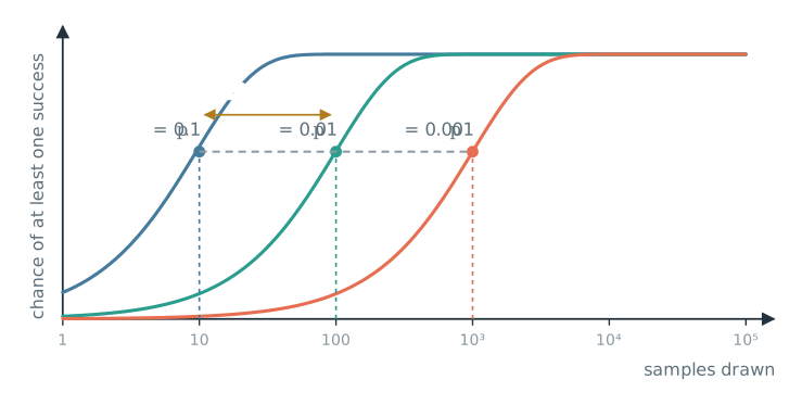
Real samples are nowhere near independent. A model that misreads a problem reproduces that misreading again and again, so the observed rate behaves more like
\[1-(1-p)^{N_{\text{eff}}}, \qquad N_{\text{eff}}\ll N,\]where $N_{\text{eff}}$ counts only the attempts that are genuinely distinct. In the worst case — a model committed to one wrong approach — every draw is the same draw and $N_{\text{eff}}=1$. This is why best-of-$N$ flattens long before the arithmetic says it should, and why diversity is a first-order term: temperature, prompt variation, forced decompositions and different checkpoints do not add samples so much as distinct ones, and only distinct ones appear in the exponent.
None of this is specific to language. Generate an image and it is almost right; generate another and the tenth one is excellent. The same holds for video, audio, design and writing.
Binary success is also the special case. Give each output a quality score $Q(y)$, let $F(q)=P(Q\leq q)$ be its distribution under a single draw, and write $Q_N^\star$ for the best score among $N$ draws. Then $P(Q_N^\star\leq q)=F(q)^N$, so $Q_N^\star$ lands around the $1-1/N$ quantile of one draw:
\[\boxed{ Q_N^\star\approx F^{-1}\!\left(1-\tfrac1N\right). }\]Pure order statistics: no reasoning, no chain of thought, no reinforcement learning. Call everything above a threshold a “success” and $1-(1-p)^N$ falls out as a corollary. Note what this does not say. It fixes the quantile the best sample lands on, not how fast quality rises — that depends entirely on the tail. A heavy tail keeps paying as $N$ grows; a tail with a ceiling stops at once.
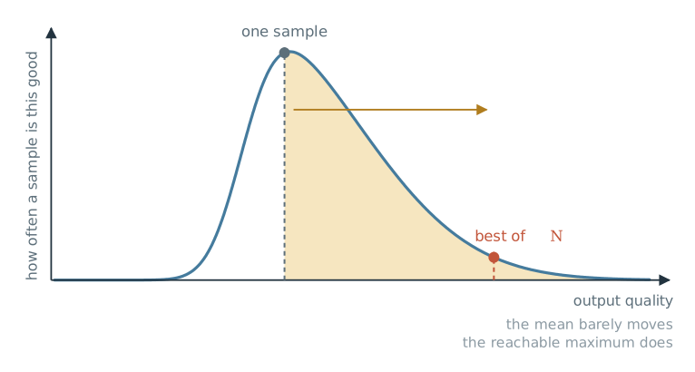
Two numbers get used interchangeably and should not be. pass@$N$, or coverage, asks whether any of $N$ samples was correct — it scores the generator, and it quietly assumes an oracle that always picks the right one out of the pile. Best-of-$N$ is what you actually receive once a real selector chooses. Oracles are not available, so best-of-$N\leq$ pass@$N$, and the gap is not noise: it is your selector’s quality, reported as a benchmark number. Latent capability and deliverable performance are different quantities, and a large pass@$N$ under a weak selector is exactly a capability you demonstrably have and cannot deliver.
Draw a thousand candidates, return one at random, and nothing improves. Someone has to know which one is good. The object is never generation alone:
\[\boxed{ \text{generation}+\text{selection}. }\]4) Why Math and Code Went First
Math and code have unusually scalable selectors. A model writes a patch: compile it, run the tests, read the stack trace. It produces a mathematical answer: check it. The evaluator is objective, cheap, and runs millions of times:
\[\boxed{\text{a scalable verifier}}\]One artifact then does four jobs: reward in training, selection at inference, evaluation, and feedback. A failed test is not only a failure. It is information, which turns flat search into a loop:
\[\text{generate}\rightarrow\text{test}\rightarrow\text{revise}\rightarrow\text{repeat}.\]Which is why I do not think coding models can be explained by reinforcement learning with verifiable rewards (RLVR) alone. RLVR is an amplifier, not a source: the base model must already propose useful algorithms, repairs and decompositions often enough to be found. Without probability mass there is nothing to select, and without a verifier there is no scalable way to find the tail.
The contrast is sharpest in open-ended work. A model can write excellent code and bland prose, because good writing has no unit test — whether a sentence actually says something is not a property you can assert. Humans judge it well, and human judgment does not scale to a million rollouts.
So the real condition is not the one usually stated. Test-time scaling does not require a task to be verifiable in any formal sense. It requires good outputs to be selectable, cheaply and often. Someone regenerating an image until one looks right runs a coding agent’s loop with taste in place of a test suite. Only the cost per selection differs, and that cost decides how far $N$ goes.
5) The Strange Part Is Where the Probability Comes From
Repeated sampling is not the mysterious part. Humans understood rare events long before neural networks. The real question is:
Why does a useful outcome have non-negligible probability in the first place?
That is what model scaling changes. A weak model may give an excellent solution $p=10^{-100}$: technically nonzero, practically nonexistent. A stronger one moves it to $10^{-3}$. Nothing about the task changed; the solution moved from an unreachable tail into a searchable region. So “the model has nonzero probability of generating the solution” is too weak a statement to mean much.
Suppose a valid proof of the Riemann hypothesis exists as a finite object. The interesting quantity is not whether a model assigns it nonzero probability but how much mass it puts on valid proofs. At $10^{-1000000}$, nothing follows. At $10^{-6}$, the problem suddenly looks like search. I am not claiming either number — the point is simpler.
The mystery is not that more samples can reveal a rare event. The mystery is that scaling prediction creates a distribution in which highly structured, useful computations become probable at all.
6) How Far Can Compute Reach?
Put this on a natural scale. With success probability $p$, write
\[D=-\log p.\]Read $D$ as a volume ratio: if the model searches among $K$ roughly equally likely lines of attack and $M$ work, then $p=M/K$ and $D=\log(K/M)$. So $D$ is not the length of the answer or the complexity of the problem. It measures how small the successful region is inside the space the model actually explores — at $D=10$ bits, about one part in a thousand of what it would otherwise produce.
Which means $D$ is a property of the pair, not of the task. The same problem has a large $D$ for a weak model and a small one for a strong model, and it shifts again with the prompt, the tools, the decoding. There is no model-independent difficulty here — only distance from a particular solver to a particular target.
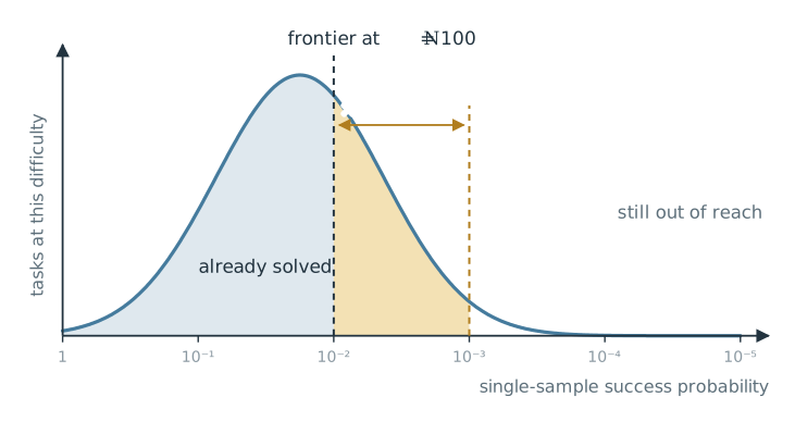
For repeated sampling, the transition happens around $Np\sim1$. Since $p=e^{-D}$, this becomes $Ne^{-D}\sim1$, and therefore
\[\boxed{ D\sim\log N. }\]Multiplicative compute buys additive reach into improbability.
Ten times the compute reaches one more decade into the tail; ten times again buys another. It also puts training and inference in the same units: training lowers $D$, inference raises the frontier $\log N$. They are not the same lever, since training reshapes the distribution while inference only spends against a fixed one, but they share an axis and in some regimes one can be traded for the other.
There is a deeper reason the two land in the same units. Cross-entropy training already measures surprisal: for a target trajectory $\tau=(y_1,\ldots,y_T)$,
\[\begin{gathered} -\log p_\theta(\tau\mid x)\\ =\sum_t -\log p_\theta(y_t\mid x,y_{\lt t}). \end{gathered}\]$D$ is the same coordinate, except that $p$ is the total mass on successful computations rather than one particular target sequence:
\[D_\theta(x)=-\log\sum_{\tau\in\mathcal{S}_x}p_\theta(\tau\mid x),\]with $\mathcal{S}_x$ the set of trajectories that solve $x$. Not the same objective as ordinary supervised training, but the same surprisal geometry. Training moves mass toward useful trajectories and lowers their surprisal; inference leaves the distribution fixed and pays exponentially more samples to reach what remains surprising.
So compute does not make every problem easier. It moves a frontier: tasks with $p\gg 1/N$ are reachable, tasks with $p\ll 1/N$ stay invisible.
7) What a Scaling Curve Is Actually Measuring
Everything so far was one task. A benchmark is a population of them, each with its own $p$, and aggregate accuracy averages many individual curves:
\[A(N)=1-\mathbb{E}_p\big[(1-p)^N\big].\]Exact, but awkward in that form. Move to the failure-exponent coordinate $r=-\log(1-p)$, so that $(1-p)^N=e^{-Nr}$. Under iid repeated sampling the average then collapses:
\[\begin{aligned} 1-A(N) &=\mathbb{E}_r\big[e^{-Nr}\big]\\ &=\int_0^\infty e^{-Nr}f_r(r)\,dr\\ &\equiv\mathcal{L}[f_r](N), \end{aligned}\]with $f_r$ the density of $r$ across the benchmark. The benchmark failure curve is exactly the Laplace transform of the distribution of per-task failure exponents. Nothing is approximated and nothing about neural networks enters: the shape belongs to $f_r$ and to nothing else.
The tasks that still matter at large budget are the hard ones, and there $p\ll1$ gives $r=-\log(1-p)\approx p$, so
\[1-A(N)\approx\mathcal{L}[f_p](N).\]That is worth saying plainly. Easy tasks drop out of the scaling problem almost immediately — a task at $p=0.5$ is finished by $N=10$ and contributes nothing afterwards. At large budgets the curve is governed by tasks near the moving frontier $p\sim1/N$ and by the harder tail beyond it. That frontier is the one we already have:
\[p\sim 1/N \quad\Longleftrightarrow\quad D\sim\log N.\]Each task’s curve is a soft step centered near $D=\log N$, so averaging them gives
\[A(N)\approx F_D(\log N),\]with $F_D$ the cumulative distribution of task difficulty: accuracy is however much of the landscape now sits behind the frontier. Since the frontier advances by a constant per decade of compute, every feature of the curve belongs to the landscape rather than to the motion.
A scaling curve is a shadow of the latent difficulty landscape.
| how difficulty is distributed | resulting curve |
|---|---|
| flat in $D$ — about as many tasks per decade of $p$ | $A(N)\sim\log N$ |
| thinning exponentially, $f_D\sim e^{-\alpha D}$ | $1-A(N)\sim N^{-\alpha}$, a power law |
| bounded hardest task | saturates and stops |
| gaps between clusters of difficulty | plateaus, then sudden jumps |
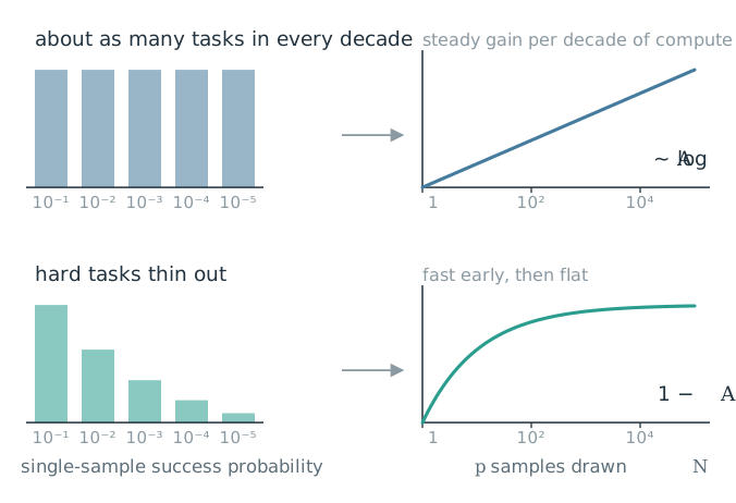
The first two rows are worth writing out. If the difficulty density is roughly flat, $f_D(D)\approx\text{const}$, then across the range where the frontier sits inside that flat region
\[A(N)\approx a+b\log N,\]which is the log-linear law everybody quotes — and it is a fact about the benchmark, not about scaling. If instead the hard tail thins exponentially, $f_D(D)\propto e^{-\alpha D}$, identical per-task exponentials aggregate into
\[1-A(N)\propto N^{-\alpha}.\]None of this is mine — the aggregation has been studied directly. What it changes is the question. We ask why a curve has its shape as though the shape belonged to the model. It belongs to the distribution underneath.
8) The Verifier Is Not an Oracle
So far I have quietly assumed an oracle selector: whenever search reaches a good answer, we know it. Real systems do not get that oracle for free. The verifier imposes a second limit, and it has the same shape as the first.
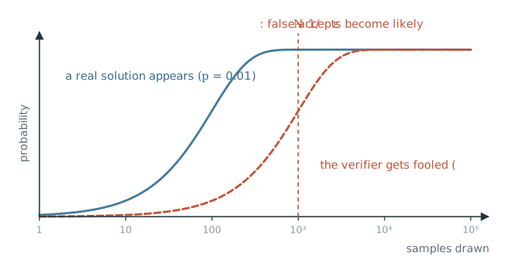
Take a deliberately crude model. A candidate is genuinely correct with probability $p$ and always accepted; a bad candidate is falsely accepted with independent probability $\epsilon$. So per draw the chance of a true accept is $p$ and of a false accept $(1-p)\epsilon$. This is a toy independent-error model, not a law — adaptive optimization exploits correlated weaknesses in a checker, hunting its blind spots, so a real search fails earlier than this suggests. But the shape shows through. Over $N$ draws the chance of a genuine solution is $1-(1-p)^N$ and the chance of at least one false accept is $1-\big(1-(1-p)\epsilon\big)^N$, which for rare success $p\ll1$ is about $1-(1-\epsilon)^N$ — the identical form. Search and self-deception scale together.
Worse, the ratio never improves. Among accepted candidates the fraction actually correct is
\[\text{precision}\;=\;\frac{p}{p+(1-p)\epsilon},\]which contains no $N$ at all. Sampling deeper does not make what you accept more trustworthy. It multiplies real solutions and convincing frauds in the same proportion.
Two different scales come out of this, and they are worth keeping apart. At $N\sim1/\epsilon$ a false accept becomes likely — but that is not a wall on useful search, since a task with $p\gg\epsilon$ still returns far more genuine solutions than frauds. The reach limit is the other comparison. An accepted output ceases to be more likely correct than incorrect once true and false accepted mass are comparable,
\[p\sim(1-p)\epsilon\;\approx\;\epsilon \qquad (p\ll1),\]so the verifier-limited reach in difficulty space is $D_{\max}\sim\log(1/\epsilon)$. It sits beside the compute frontier in the same units and the same form:
\[\boxed{ D\sim\log N \quad\text{and}\quad D_{\max}\sim\log\tfrac{1}{\epsilon}. }\]Compute decides how deep you can look; the verifier decides how deep you can trust. The smaller one binds. A checker with a $1\%$ false-accept rate cannot certify anything much rarer than one in a hundred, however much compute you point at it — that is reward hacking stated quantitatively, and why so much effort goes into stricter verification rather than better generation.
There is a familiar analogy to certificate verification: for many problems, checking a proposed solution can be much easier than constructing one, and that gap is the whole reason generate-and-select exists. Guessing a certificate of length $n$ uniformly puts $D$ at $n\log\lvert\Sigma\rvert$ — the brute-force wall. Pretraining does not change the worst-case complexity class of the underlying formal problem; it changes the proposal distribution, often making useful certificates vastly less surprising than uniform guessing. On the instance distributions we actually care about, that change can dominate everything else.
The idealization also assumes a sound checker, one that never accepts a wrong answer: $\epsilon=0$, so $D_{\max}=\infty$. Real verifiers rarely are. Formal proof is an unusually clean example of a sound checker, and other exact or narrowly specified verification settings exist too. Everywhere else $\epsilon>0$ sets the ceiling.
9) Why Long-Horizon AI Does Not Immediately Collapse
A verifier can do more than choose among finished samples. Generation produces uncertainty over possible trajectories; verification turns an outcome into information. Feed that information back into the context and the next distribution is no longer the one you started with:
\[p_\theta(a_{t+1}\mid h_t) \;\longrightarrow\; p_\theta(a_{t+1}\mid h_t,v_t),\]with $v_t$ whatever the verifier or the environment returned. Selection acts on a distribution after the fact; feedback acts on the next one. Generation creates possibilities, verification makes them informative, and feedback spends that information on what gets generated next — which is how a closed loop can reduce the difficulty of the search that remains instead of only paying for more of it.
An old intuition seems to contradict all of this. If each reasoning step is correct with probability $q$, then over a chain of length $L$,
\[P(\text{all steps correct})=q^L,\]which collapses exponentially. Shouldn’t long chains of thought and long-horizon agents be hopeless?
The equation is fine; it measures the wrong event. It demands one unbroken chain with every step correct forever — the right model for an open loop. Modern systems run closed ones: they branch, restart, call tools, check intermediate results, notice contradictions, repair. The useful quantity is not
\[P(\text{never make a mistake}),\]but
\[P(\text{success within the budget}).\]In an open loop an error is damage. In a closed loop it can become information: a wrong patch plus a failed test leaves the system knowing more than before. Error accumulation does not vanish — a model can equally condition on its own mistake and grow more confident in something wrong. Two forces compete, and external feedback gives the second a chance. Which is again why verifiable environments scaled first.
In the coordinate we already have, the distinction is sharp. Repeated sampling holds $D$ fixed and buys more $\log N$: the task never gets easier, you just look longer. A closed loop is different — every observation that rules something out shrinks the space still worth searching, so difficulty itself falls as the system works:
\[D_0>D_1>D_2>\cdots\]That is the real difference between an agent and a large batch of samples, and why one with a working feedback channel can beat best-of-$N$ at equal token cost. It is not merely buying more search capacity; it is spending compute to reduce the search required.
The same two coordinates say something about multi-agent systems, which are the obvious way to spend a large budget. More agents are not automatically more useful compute; what matters is which term the orchestration actually moves.
\[\begin{array}{ll} \text{independent proposals} & N_{\text{eff}}\uparrow\\ \text{informative feedback} & D\downarrow\\ \text{correlated imitation} & N_{\text{eff}}\downarrow\\ \text{misleading feedback} & D\uparrow \end{array}\]Parallel agents help when they genuinely explore different hypotheses, and specialized ones when they contribute computation or evidence the rest do not have; a test, a tool or an environment helps because it returns something no agent already contained. Free-form discussion is the case to watch. Agents sharing one model prior begin conditioning on each other’s mistakes and converge on a common answer, so the disagreement that made the ensemble worth running disappears while the uncertainty about the truth stays exactly where it was.
A good multi-agent system converts parallel uncertainty into information. A bad one converts independent errors into correlated confidence.
10) The Tail Becomes the Mode
If expensive inference can repeatedly discover rare successful trajectories, the obvious next move is to train those discoveries back into the model. Training and inference sit on the same axis, after all — whatever search finds at great expense can be trained back in cheaply.
A useful behavior occurs with probability $10^{-4}$. Search finds trajectories that do it. Train on them, and the next model produces it at $10^{-1}$. What once took thousands of attempts now happens routinely, and the freed compute goes looking for something rarer.
Search the tail. Learn from what works. Move it toward the mode. Search farther.
Which is why synthetic data gets more interesting as models get stronger: a weak model feeding on itself reproduces its weaknesses, while a strong one with search and verification generates signal that is better targeted and harder. AI stops being only the product of the training pipeline and starts producing the next one.
The objection to this loop is the most important open question here. If search only surfaces trajectories the model could already produce, training on them may simply re-weight the distribution rather than expand the reachable frontier. Mass moves toward what worked: sharper, not necessarily wider.
Though “wider” needs care. A softmax model already puts positive probability on almost every finite token sequence, so nothing is literally outside its support. What matters is the effective support: outcomes carrying enough mass to be reached on a real budget. Sharpening raises $p$ on behavior that is already reachable. Sharpening alone must eventually saturate; continued progress requires moving the reachable frontier.
This is measurable, uncomfortably so. RLVR often improves pass@1 and can lower pass@$k$ at large $k$: the model grows likelier to hand you its best answer first and less likely to hand you a hundred genuinely different ones. Concentration and coverage trade off — exactly what you would expect if training were redistributing mass rather than creating it.
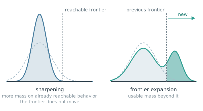
If the loop only sharpens, it converges: you cash out the tail you had, faster each round, and then run out of tail. Sustained frontier expansion requires more than repeatedly reweighting the same discovered successes. In current systems the clearest sources of new signal come from tools, environments, experiments, fresh data, or people — a tool that computes what the model cannot, an environment that answers a question its training data never asked, a person who poses a problem nobody had posed.
This is why I would hesitate to call the current loop open-ended recursive self-improvement. The feedback structure is real — better model, better search and data, better model again — and it is already doing a great deal. But sharpening what a model can already reach is not the same claim as open-ended expansion of what it can reach, and only the first of those looks established.
11) It Just Works
In the simple picture above, everything collapses into one inequality. With $D_\theta(x)=-\log p_\theta(x)$ as above, $p_\theta(x)$ being the model’s single-attempt success probability on task $x$, that task becomes practically reachable when its difficulty falls under both ceilings at once:
\[\boxed{ \underbrace{D_\theta(x)}_{\text{training}} \;\lesssim\; \min\Big( \underbrace{\log N}_{\text{inference}} ,\; \underbrace{\log\tfrac1\epsilon}_{\text{verification}} \Big) }\]The three roles from the beginning now sit on the same reachability axis. Cross-entropy training, inference scaling and verification look like different parts of the stack, but in this picture they trade in the same currency: surprisal. Training lowers $D_\theta(x)$ by making success less surprising; inference raises $\log N$, paying for reach; verification sets $\log(1/\epsilon)$, the depth at which that reach can still be trusted. Because the right side is a minimum, the weakest of the three decides everything. A closed loop is the case where the left side falls while the system works, and successful search becomes training data that lowers it again next round.
When I first used ChatGPT I had no theory for why it felt different, only the intuition that it was not ordinary autocomplete. That reaction has not worn off. What changed is that I now have some idea what I was reacting to — and what surprises me is how little exotic machinery it takes.
Maybe there is no single trick that turns prediction into intelligence. Maybe the remarkable thing is that a good enough learned distribution already holds an enormous space of useful computations, and that operations as generic as sampling, search, feedback and selection are enough to exploit it.
And somehow, AI just works. I still find that remarkable.
Yufa Zhou — September 3, 2026